Keywords: Gaussian Mixture Models, GMM, cluster, Expectation-Maximization, EM

In a previous post, I went through job advertisements and clustered them using K-means to create groups of similar job advertisements. I looked at job advertisements for “data scientist”, and K-means created clusters. Without any prior information, Kmeans recovered clusters with financial, health or developer focus. However, there are many advertisements that either do not have a clear focus, or may be an intersection of two or more clusters.

Clustering with Gaussian Mixture Models (GMM) allows to retrieve not only the label of the cluster for each point, but also the probability of each point belonging to each of the clusters, and a probabilty distribution that best explains the data. This has many practical advantages. In the job advertisement classification example, this allows to focus on the jobs in cluster \(i\), but also to take into consideration job advertisements that belong primarily to another cluster, but still have a probability of belonging to cluster \(i\).

Gaussian Mixture Models are used beyond clusering applications, and are useful model fitting techniques as they provide a probability distribution that best fits the data. The algorithm that allows to fit the model parameters is known as Expectation Maximization (EM).

After a short introduction to Gaussian Mixture Models (GMM), I will do a toy 2D example, where I implement the EM algorithm from scratch and compare it to the the result obtained with the GMM implemented in scikit. Finally, we can apply the GMM to cluster the job advertisements.

Gaussian Mixture Models

If we have a strong belief that the underlying distribution of univariate random variable \(x\) is Gaussian, or a linear combination of Gaussians, the distribution can be expressed as a mixture of Gaussians:

where \(\pi\) is a vector of probabilities, which provides the mixing proportions. In the multivariate case,

where \(\vec{x} \in \mathcal{R}^N, \vec{\mu} \in \mathcal{R}^N, \Sigma \in \mathcal{R}^N \times \mathcal{R}^N\). The goal of modelling is to find (learn) the parameters of the GMM: weights, mean and covariance. The covariance matrix \(\Sigma\) is symmetric positive definite and thus contains \(N(N+1)\) free parameters. To reduce the number of parameters, the off diagonal terms may be set to zero, and only the variance in each dimension is fitted, reducing it to \(N\) parameters.

Clustering using Gaussian Mixture Models

Let \(z_i\) be the cluster label of random variable \(\vec{x}_i\) which is hidden from us. For this reason, \(z_i\) is sometimes referred to as a hidden or latent variable.

In a mixture model, we first sample \(z\), and then we sample the observables \(x\) from a distribution which depends on \(z\):

\(p(z)\) is always a multinomial distribution, and \(p(x \| z)\) is, in general, any distribution. In the special case of Gaussian Mixture Models, \(p(x \| z)\) is Gaussian. We can obtain \(p(x)\) by marginalising over \(z\),

In the clustering case, for each point \(x_i\):

If we have \(N\) points that are i.i.d , and \(p(x\|z)\) Gaussian,

The Expectation-Maximization (EM) algorithm is used to iteratively update the model parameters and the values of the latent variables (cluster labels). The two steps in the EM algorithm are repeated iteratively until convergence (i.e: no changes in responsibility vectors):

• Expectation step: With the prior for the model parameters, we want to compute a posterior on the cluster probability for each point ( \(p(z_i = k \| x_i, \pi_k, \mu_k,\Sigma_k)\)) sometimes also called responsibility vector.

  Recalling Bayes Theorem,

we can use it to compute the posterior probability we are interested in:

​
Note that \(\gamma_{i,k}\) denotes the probability that point \(x_i\) belongs to cluster \(k\). This allows to quantify the incertitude on the cluster labelling. For example, if there are 3 labels and \(\gamma_{i,k} = 1/3\) means the labelling has a lot of incertitude.

• Maximisation step: To find the optimal parameters \(\mu, \Sigma\), we need to maximise the log-likelihood of \(p(x)\). The log likelihood is:

To maximize it, we need to find \(\partial \mathcal{L} /\partial \mathcal{\mu}\) and \(\partial \mathcal{L} /\partial \mathcal{\Sigma}\). If it can’t be done analytically, a numerical optimization would have to solved. In the case we are dealing with which is a mixture of Gaussians, a closed solution is possible, and can be shown to be:

where

To go through the clustering algorithm using a Gaussian Mixture Model, let’s first do a toy example with two dimensions. Afterwards, we will use GMM to cluster the Indeed job advertisements.

Gaussian Mixture Model : a toy example.

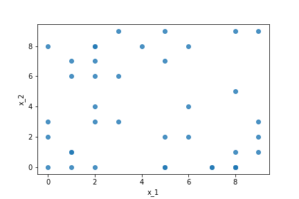
We have \(N=40\) points, in two dimensions, and we would like to find and underlying structure with \(k=3\) clusters.

We will:

1. Write the EM algorithm from scratch
2. Compare the outcome with the built in GMM from scikit sklearn.mixture.GaussianMixture

You can download the notebook here.

There are two main functions that will be called iteratively.

• In EM, the first step is the expectation step where we compute equation (1) which is the posterior of the probabilities of each point belonging to a cluster:

def compute_post(m,k,x,mu,sigma, prior_cl):
    PostZ = np.zeros([m,k])
    for ix,iv in enumerate(x):   #for each data point
        for ik in range(k):      # for each cluster 
            PostZ[ix,ik] = prior_cl[ik]*multivariate_normal.pdf(iv, mean=mu[ik], cov=sigma[ik])
        nc = sum(PostZ[ix,:])    #normalize by sum of row
        PostZ[ix,:]= PostZ[ix,:]/nc
    return PostZ

• In the maximization step, we update the parameters of the GMM

def update_params(m,k,x,mu,sigma, PostZ):
    # 1. Update priors
    for ik in range(k): 
        prior_cl[ik] = np.mean(PostZ[:,ik])

    if (abs(sum(prior_cl)-1) >0.001) : 
        print('Something went wrong: priors dont sum to one')

    #2. Update mean
    nk = [0 for i in range(k)]
    for ik in range(k): #Update mean of each cluster : weighted average
        nk[ik] = np.sum(PostZ[:,ik])
        mu[ik] = np.sum(np.reshape(PostZ[:,ik],[len(x),1])*np.array(x), axis=0)/nk[ik]
        #print(mu[ik])

    #3. Update Variance 
    for ik in range(k):
        sigma[ik][0,0],sigma[ik][1,1]= np.sum(np.reshape(PostZ[:,ik],[len(x),1])*(np.array(x)-mu[ik])*(np.array(x)-mu[ik]),axis=0)/nk[ik]

    return prior_cl, mu, sigma

Now, we can call EM steps iteratively,

mu, sigma, prior_cl = init_mu_sigma(k,N,x, debug=0)
mu0 = copy.deepcopy(mu)
for it in range(100):     
    Postz = compute_post(m,k,x,mu,sigma, prior_cl)
    prior_cl, mu, sigma = update_params(m,k,x,mu,sigma, Postz)
hard_labels = np.argmax(Postz, axis=1)

The matrix Postz has dimensions \(N \times k\) where entry Postz[i,j] represents the probability that point \(x_i\) belongs to cluster \(k\).

GMM in Python with sklearn

The sklearn.mixture package allows to learn Gaussian Mixture Models, and has several options to control how many parameters to include in the covariance matrix (diagonal, spherical, tied and full covariance matrices supported). sklearn.mixture.GaussianMixture uses Expectation-Minimization as previously explained. Using this function, the clustering with GMM is simply:

estimator = GaussianMixture(n_components=k,
                   covariance_type='diag', max_iter=20, random_state=0)
estimator.fit(x)               # Learns model parameters
label = estimator.predict(x)   # predicts label for each point
y_prob = estimator.predict_proba(x) 
#y_prob is the responsability matrix: the probability of each point being in each cluster.

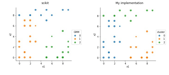
The clustering results are shown below. On the left is using the scikit function, and on the right the implementation from scratch sketched above.

The colors indicate clusters, and the sizes are proportional to the certainty. Both functions arrive to nearly same results always, although sometimes a few points may differ. The implementation without using scikit was mainly to test my understanding.

Clustering job advertisement with GMM

We can now use GMM to cluster the Indeed Jobs. You can download this notebook.

As I did in my previous post, I collected the job advertisements for “data-scientist”, and created the features using TF-IDF. All the pre-processing is exactly the same, so I will not repeat the details.

After clustering, I look at where the centres of the Gaussians are, and look the ones that have the most weight, to understand each cluster. For a specific run, the results were as follows:

Important features for cluster  0
research                      0.13519889107029157
sciences                      0.09332351293807206
social                        0.08184207446558818
data                          0.0771361762386771
content                       0.07563418282231256

 
 Important features for cluster  1
analyst                       0.1040533220599665
analytics                     0.09383322420589418
business                      0.08764275289464411
data                          0.08016894058385425
customer                      0.07747423994838035

 
 Important features for cluster  2
business                      0.060880200267596746
data                          0.0602169703252302
engineer                      0.0595723383638893
help                          0.056738072390410184
projects                      0.05558856031452268

 
 Important features for cluster  3
developer                     0.16206101848635407
software                      0.12119626940241453
java                          0.11103844485126925
selection                     0.10707740528104592
coding                        0.0893526401058581

Let us now look in detail at the certainty of each job advertisement classification

As mentioned, estimator.predict_proba(features) returns a \(N\times k\) matrix, representing the probability that advertisement \(x_i\) belongs to cluster \(k\). Here is an example of the first ten advertisements:

[[  4.91272164e-42   1.47300082e-01   8.24583506e-36   8.52699918e-01]
 [  1.72533774e-62   9.99947673e-01   5.00420735e-53   5.23273617e-05]
 [  8.55562609e-43   1.23105622e-01   4.17968854e-37   8.76894378e-01]
 [  5.92908971e-54   9.97533813e-01   8.29750436e-46   2.46618681e-03]
 [  4.39147798e-03   4.13869091e-45   9.95608522e-01   3.24111757e-28]]

So, for example, the advertisement on the first row belongs primarily to cluster 3, but can also be in cluster 1. The job advertisement in the second row is mostly in cluster 1, and advertisement in the third row can belong to both cluster 1 and cluster 3.

Clustering in this way can allow you to better target what you are looking for, and loose valuable information that, although being more likely in another group, may still be useful in your search.

Remarks

I have deliberately left out the discussion on feature selection and selecting the number of clusters. In a supervised setting, we would do cross validation to select these. For the unsupervised setting, this topic will be discussed in a later post.