How can we teach a computer to play games? The first thing we need is a way to represent game states. Trees are common data structures used for game representations. Every node in a tree is a possible game board (state), and child nodes are possible game actions.

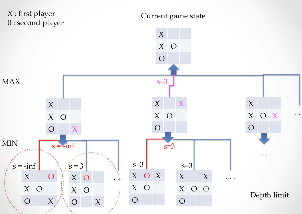
The root of a tree is the representation of the initial game state. The intial state could be, for example, an empty board, or a board somewhere along the game. Consider two players denoted by \(P0\) and \(P1\). In the figure above, the first player is trying to decide the fifth action of the game (his third action). Suppose there are \(b_1\) possible moves for player \(P0\). The first level of a tree will contain \(b_1\) nodes (possible actions), and player \(P0\) will try to maximize his chance of winning with that action. For each node \(b_1\), \(P1\) has, for example, \(b_2\) possible actions. In the next game turn, at level 2, player \(P1\) will try to minimize the chance of \(P0\) winning. As we move down the tree, taking turns between player \(P1\) and player \(P2\), the function that evalutes the probablity of player \(P1\) winning is being maximized, then minimized, in an alternating fashion

Minimax algorithm:

Once all the possible game states have been played to end game, it is possible to see some branches lead to \(P0\) winning the game. How can the information about the outcome of the game be propagated up to the first depth of the tree to choose a first action? This is where we make use of the minimax algorithm.

If the game end resulted in a failure for player \(P0\), a value of \(v=-\infty\) (for example) is assigned to that leaf, as shown in the leftmost branch of the figure. On the contrary, if the game end resulted in a win for player \(P0\) a value of \(v=+\infty\) is assigned to that leaf. If at a certain depth the player has not won or lost, and we cannot explore deeper possibilities, then a score is assigned to the board. The values \(v\) of each leaf are then propagated up the tree, by selecting the minimum/maximum (mini-max) value among the child nodes, at each node moving up the tree, until we reach the root. Moving up the tree with mini-max ensures that \(P0\) chooses a branch that maximizes his outcome and \(P1\) chooses a branch that minimizes the outcome of his opponent. When we reach the root, \(P0\) will know which is(are) the first best move(s) of the branches he analyzed. There are great tutorials and lectures out there. This blog has a long clear tic-tac-toe example. .

A first approach in creating a game playing agent, is to create a tree with all possible moves and use the minimax algorithm to determine which action to take at each level. This requires to visit all nodes in a tree. How many nodes are there for a tree with a specific depth and branching factor ?

Nodes in a tree :

Imagine a tree with a branching factor of \(b=3\). At level zero there is one node. At level 1, \(3\) nodes are added. At level two, \(9\) nodes are added. The sum of all nodes in a tree is

\[\begin{equation} S_d = \sum _{i=0}^{i=d} 3^i = 1 + ... + 3^d \tag{1}\label{eq:sd} \end{equation}\]

To find \(S_d\), multiply equation (1) by 3,

\[\begin{equation} 3 s_d = \sum _{i=0}^{i=d} 3^i = 3 + ... + 3^{d+1}, \tag{2}\label{eq: 3sd} \end{equation}\]

and subtract (1) from (2). The total number of nodes in a tree of depth \(d\) with branching factor \(3\) is,

\[S_d = \frac{3^{d+1}-1}{2}.\]

In general, for a tree with branching factor $b$, the total number of nodes is

\[S_d = \frac{b^{d+1}-1}{b-1}.\]

Searching for a good gaming strategy can rarely be done by brute force by visiting all the nodes, because we can see that the number of nodes grows exponentially with the depth of the tree (\(O(S^d) = b^d\)). Therefore, we have to limit the depth of the search.

Depth limited search:

The number of nodes to be visited is of the order of \(n = b^d\) where \(b\) is the branching factor and \(d\) is the depth. Assume a computer can perform \(T_0 = 10^9\) operations per second, or can visit \(10^9\) nodes per second. If the maximum time searching for a next move is \(T = k T_0\) , then \(b^d < T\). Therefore, the maximum depth that can be searched in this time is \(d < \frac{\log_{10} T}{\log_{10}{b}}.\)

Static evaluation/Evaluation function/scoring function:

At level \(d\), the algorithm has to assume each node is a leaf, and score each node with a function that is indicative of the probability of success if the game were to continue down that branch. A static evaluator (or evaluation function) is used to score each node and make a decision at this level. Designing the right static evaluator is tricky. Static evaluators should be:

• fast : If it takes longer to compute the evaluation function, than to search one level deeper, then in some games it may be better to search one level deeper.
• accurate: Although short in compute time, the static evaluator should capture the chance of success for each node.

Quiescent search:

When the recommended branches given by the evaluation function vary wildly when the depth of the search is changed, then it may be an indication that search to deeper levels needs to be done. When searching to deeper levels in the tree, the recommended branches stay mainly the same, then a state of quiesence is achieved.

Iterative deepening:

Fixing the limit of the depth search in advance, for the entire game, may not be the best strategy. For example, the branching factor is not the same at each depth, and there may be situations where a number of branches can be discarded, leaving extra time to search deeper on the remaining branches. Therefore, rather than specifying the depth for each search, it is better to limit the time for each search (although, it may also worthwhile to consider variable time search limits depending on the stage of the game).

With iterative deepening, the algorithm searches a tree of depth 1, scores the branches with the static evaluator, and returns the next best action. If there is still time, it will now search to depth 2, and return the best action. If the time expires before it finished searching to depth 2, it will return the best action of the search with depth 1. The search will continue increasing the depth until the time expires, and always has a recommendation of best action.

Doing an iterative search to depth \(d\), the nodes in depths \(< d-1\) have been been visited several times. The nodes at depth 0 have been visited \(d\) times, the node at depth 1 have been visited \(d-1\) times, and so on. This may seem like a very costly procedure, so let’s estimate the cost.

Recall that searching ONE tree to depth \(d\) with branching factor \(b\), we have to search through \(S_d= (b^{d+1}-1)/(b-1) \approx b^d\) nodes. Note that most of the nodes (\(b^d\)) are on the last level.

The number of nodes \(I_d\) to visit if we do iterative deepening and search through ALL trees of depths in the interval \(\in [0,d]\) would be

\(I_d =S_0 + S_1 + S_2 + S_d \approx 1+b+b^2+…+b^{d-1}+b^{d}\).

Note that \(O(S_d) = b^{d}\) and \(O(I_d) = b^{d}\), so searching through ONE tree of depth \(d\) or iteratively searaching through all trees until a tree of depth \(d\) has the same computational complexity since most the compute time is spent on the last level.

Vocabulary

• Depth-First-Search (DFS): explores a path all the way to a leaf before backtracking and exploring another path. For example, you can print the values of a tree using DFS in three different ways:

  • Pre-order : print current node, go to left node and print, backtrack, go to right node and print.

  • In-order: Traverse the tree to the lefmost child and print it first. Backtrack and print. Traverse the tree to the rightmots child, and print it.

  • Post-order: Traverse the tree and find the leftmost child and print it. Backtrack. Traverse the tree to the rightmost child and print. Backtrack and print it.

Let’s play

Let’s use minimax and iterative deepening to create two agents to play matches against each other. I am also using alpha-beta pruning which is a way to discard exploring some branches to save some computational time (example 1 and 2). The game tree is visited using depth first search. When using iterative deepening, however, the search is more similar to breadth first search.

We willl play games where we have complete information.

The playing agent is provided :

• with information on possilble actions
• condition to end game
• condition to win game.
• the static evaluation function

Game 1 : Tic-tac-toe

• Possible actions: players can place themselves in any empty space.
• The game ends if a player wins, or if there are no more empty spaces.
• A player wins if it has placed itself in three positions which are in a straight line.

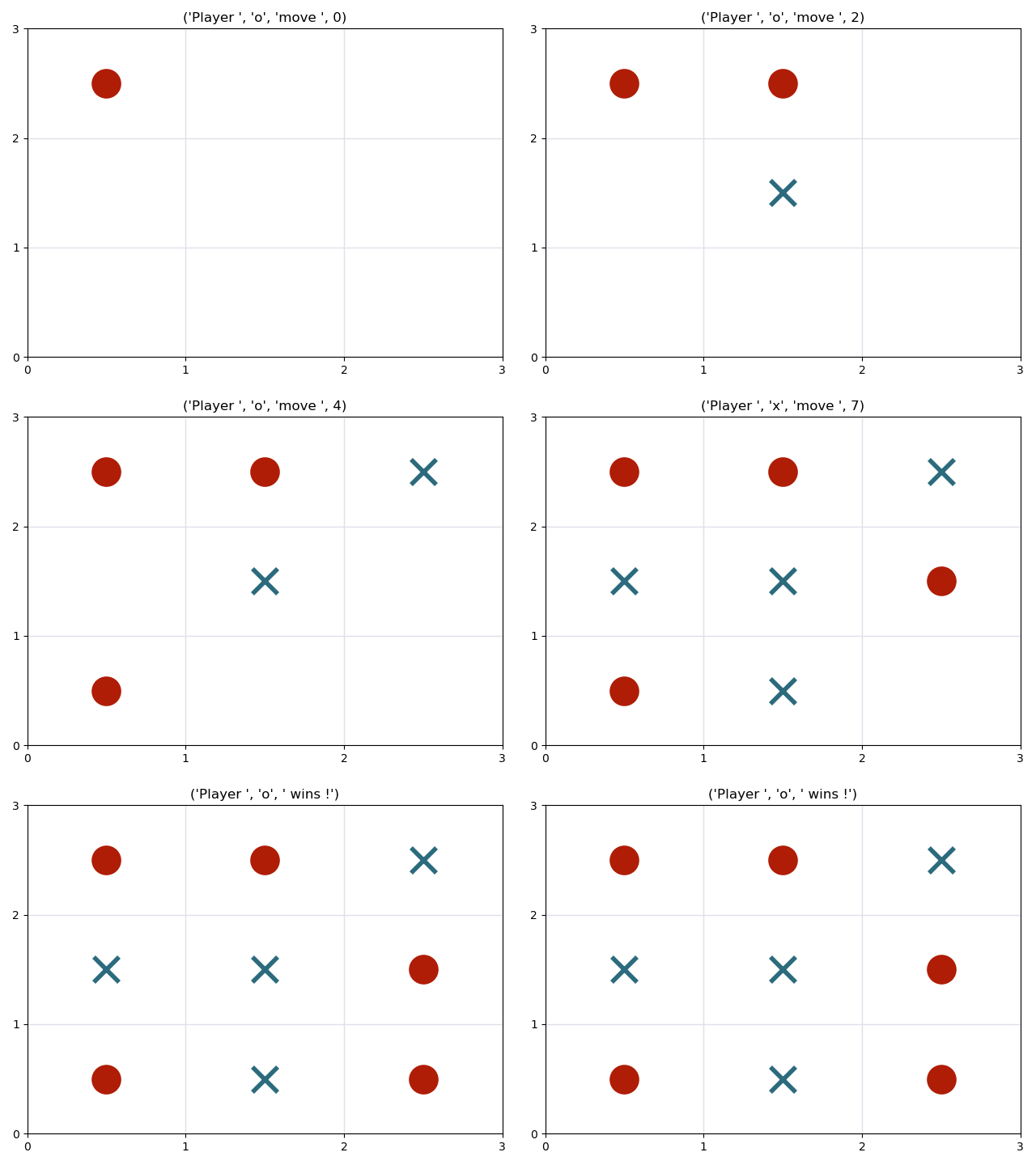
Two playing agents will play a match against each other. Both players have no time limit, and will choose one of the best moves for them. Since both players are using minimax to evaluate their best move, there is always a tie. Watch them play:

If time limits are introduced, players cannot evaluate all their moves, and will start making mistakes.

Game 2: Isolation

• Possible actions : For the first move, players can place themselves in any empty box. For further moves, players can move like a horse in chess. That is, players can move in \((\pm2,\pm1)\) or \((\pm1,\pm2)\)
• Condition to end game: The game ends if a player looses. A player looses if it has no places to move on the board.
• Condition to win the game: A player wins the game if his opponent looses.
  
  Watch a match with restrictive time limit, on a \(5\)x\(5\) board: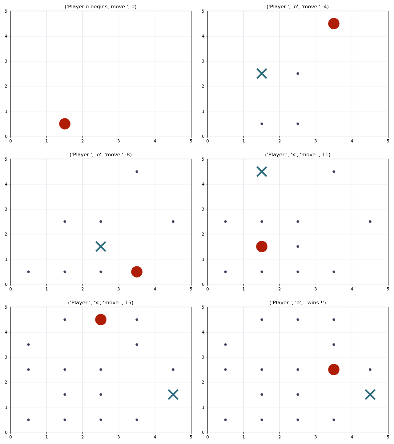
  
  Watch a match with restrictive time limit, on a \(7\)x\(7\) board: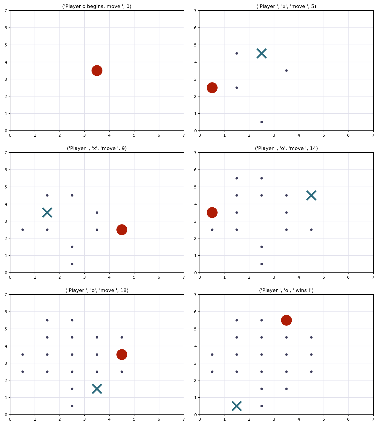

More games….

In these games there is no learning involved. At each turn, the playing agents use exclusively the mini-max algorithm to evaluate their possiblilities and choose an action. To read about games where the agents learn, check out the 2016 Nature article on AlphaGo by DeepMind.